Estimating tax payable

In this example we are given the following scenario:

Personal tax (before deductions) in Australia is based on the table below. The tax payable at the end of the financial year depends on the individual’s income. The higher the income, the higher the tax rate, as defined by tax brackets (or tiers). Given a list of incomes, calculate the corresponding tax payable for each income.

Income Thresholds	Rate	Tax payable
$0 - $18,200	0%	Nil
$18,200 - $45,000	19%	19c for each $1 over $18,200
$45,000 - $120,000	32.5%	$5,092 plus 32.5c for each $1 over $45,000
$120,000 - $180,000	37%	$29,467 plus 37c for each $1 over $120,000
$180,000 and over	45%	$51,667 plus 45c for each $1 over $180,000

We start by importing pandas, numpy and piso, and creating an interval index for the tax brackets.

In [1]: import pandas as pd

In [2]: import numpy as np

In [3]: import piso

In [4]: tax_brackets = pd.IntervalIndex.from_breaks(
   ...:     [0,18200,45000,120000,180000,np.inf],
   ...:     closed="left",
   ...: )
   ...: 

In [5]: tax_brackets
Out[5]: IntervalIndex([[0.0, 18200.0), [18200.0, 45000.0), [45000.0, 120000.0), [120000.0, 180000.0), [180000.0, inf)], dtype='interval[float64, left]')

With each interval in the tax bracket, we’ll associate three values:

1. the lower threshold for the tax bracket

2. the fixed amount payable

3. the tax rate for each dollar above the threshold (as a fraction)

We describe this data as a pandas.DataFrame indexed by tax_brackets.

In [6]: tax_rates = pd.DataFrame(
   ...:     {
   ...:         "threshold":tax_brackets.left,
   ...:         "fixed":[0, 0, 5092, 29467, 51667],
   ...:         "rate":[0, 0.19, 0.325, 0.37, 0.45],
   ...:     },
   ...:     index = tax_brackets,
   ...: )
   ...: 

In [7]: tax_rates
Out[7]: 
                      threshold  fixed   rate
[0.0, 18200.0)              0.0      0  0.000
[18200.0, 45000.0)      18200.0      0  0.190
[45000.0, 120000.0)     45000.0   5092  0.325
[120000.0, 180000.0)   120000.0  29467  0.370
[180000.0, inf)        180000.0  51667  0.450

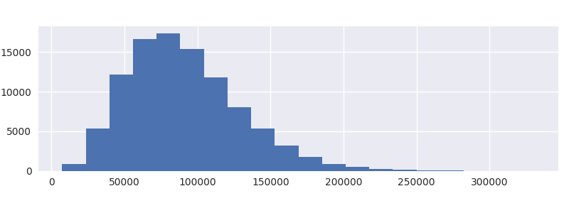
For the income, we’ll generate some random integers (and plot the distribution) corresponding to 100,000 individuals.

In [8]: income = pd.Series(np.random.beta(5,50, size=100000)*1e6).astype(int)

In [9]: income.plot.hist(bins=20);

We are now in a position to use piso.lookup(), which take two parameters:

1. a pandas.DataFrame or pandas.Series which is indexed by a pandas.IntervalIndex

2. the values which are will be compared to the interval index

In [10]: tax_params = piso.lookup(tax_rates, income)

In [11]: tax_params
Out[11]: 
        threshold  fixed   rate
61371     45000.0   5092  0.325
56606     45000.0   5092  0.325
115348    45000.0   5092  0.325
39578     18200.0      0  0.190
48203     45000.0   5092  0.325
...           ...    ...    ...
38366     18200.0      0  0.190
146076   120000.0  29467  0.370
67726     45000.0   5092  0.325
20210     18200.0      0  0.190
60895     45000.0   5092  0.325

[100000 rows x 3 columns]

The result is a dataframe, indexed by the values of income, sharing the same columns as tax_rates.

We can then use a vectorised calculation for the tax payable:

In [12]: tax_params["fixed"] + (tax_params.index-tax_params["threshold"])*tax_params["rate"]
Out[12]: 
61371     10412.575
56606      8863.950
115348    27955.100
39578      4061.820
48203      6132.975
            ...    
38366      3831.540
146076    39115.120
67726     12477.950
20210       381.900
60895     10257.875
Length: 100000, dtype: float64

Alternative approaches

There are a couple of alternative, straightforward solutions which do not require piso which we detail below.

Alternative 1: pandas.cut

The tax_params dataframe that was produced above by piso.lookup() can be reproduced using pandas.cut() which can be used to assign bins to data with an interval index.

In [13]: tax_params = tax_rates.loc[pd.cut(income, tax_brackets)].set_index(income)

In [14]: tax_params
Out[14]: 
        threshold  fixed   rate
61371     45000.0   5092  0.325
56606     45000.0   5092  0.325
115348    45000.0   5092  0.325
39578     18200.0      0  0.190
48203     45000.0   5092  0.325
...           ...    ...    ...
38366     18200.0      0  0.190
146076   120000.0  29467  0.370
67726     45000.0   5092  0.325
20210     18200.0      0  0.190
60895     45000.0   5092  0.325

[100000 rows x 3 columns]

This approach however runs approximately 20 times slower than piso.lookup().

Alternative 2: applying function

The second approach involves writing a function which takes a single value (an income for an individual) and returns the tax payable. The function can then used with pandas.Series.apply

In [15]: def calc_tax(value):
   ....:     if value <= 18200:
   ....:         tax = 0
   ....:     elif value <= 45000:
   ....:         tax = (value-18200)*0.19
   ....:     elif value <= 120000:
   ....:         tax = 5092 + (value-45000)*0.325
   ....:     elif value <= 180000:
   ....:         tax = 29467 + (value-120000)*0.37
   ....:     else:
   ....:         tax = 51667 + (value-180000)*0.45
   ....:     return tax
   ....: 

In [16]: income.apply(calc_tax)
Out[16]: 
0        10412.575
1         8863.950
2        27955.100
3         4061.820
4         6132.975
           ...    
99995     3831.540
99996    39115.120
99997    12477.950
99998      381.900
99999    10257.875
Length: 100000, dtype: float64

This approach runs approximately 3 times slower than piso.lookup(). It also requires a function to be defined which is relatively cumbersome to implement. This approach becomes increasingly unattractive, and error prone, as the number of tax brackets increases.